Usage

HornSchunck() class is written in Python. It returns optical flow velocities (u,v) for given parameters:

• alpha : (float) the regularization coefficient of smoothness constraint
• maxIter : (int) maximum number of iterations required to obtain flow velocities
• applyGauss : (bool) apply Gaussian smoothing as a preprocess {False by default}
• GaussKernel : (tuple) Gaussian Filter kernel size {(15,15) by default}

Initialize an object of HornSchunck() class with an arbitrary name, optFlow() is suggested.

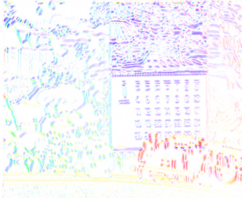
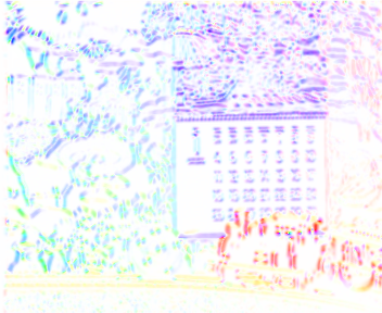
 optFlow = HornSchunck(alpha=alpha,maxIter=maxIter)
 optFlow.applyGauss  = True 
 optFlow.GaussKernel = (5,5)

Then use estimate() method to calculate optical flow velocities (u,v). After execution, getFlowField() method returns the colorized flow field.

 (u,v) = optFlow.estimate(frame1,frame2) 
 flowField = optFlow.getFlowField() 

Prediction of target frame from anchor via flow velocities is possible with predict() method. Moreover, getCollage() method puts 4 frames together to show a collage.

 anchorP = optFlow.predict() 
 collage = optFlow.getCollage(f1_idx,f2_idx)

Implementation Details

• Gaussian smoothing process is added as an optional preprocessing and highly recommended to apply to obtain better visual saturation on the flow field.
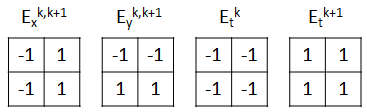
• While calculating the image and temporal derivatives Ex, Ey, Et below filters are used as a 2D convolution operands.



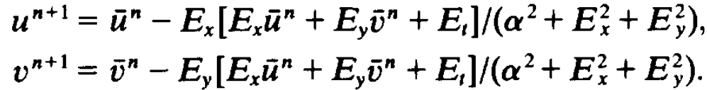
• The flow field velocities u and v are initialized with all zero matrices with a same shape of first given frame.
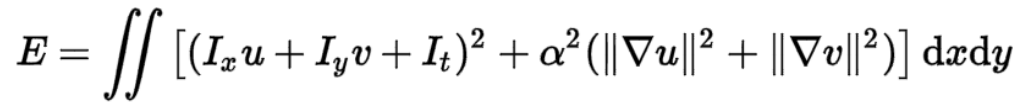
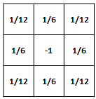
• Another 3x3 filter is used for the estimation of the Laplacian of the flow velocities as proposed in the reference paper. [1]



• New set of velocity estimates are computed from the estimated derivatives and the average of the previous velocity estimates. Also, smoothing parameter (alpha) placed in the denominator of this iterative update rule.



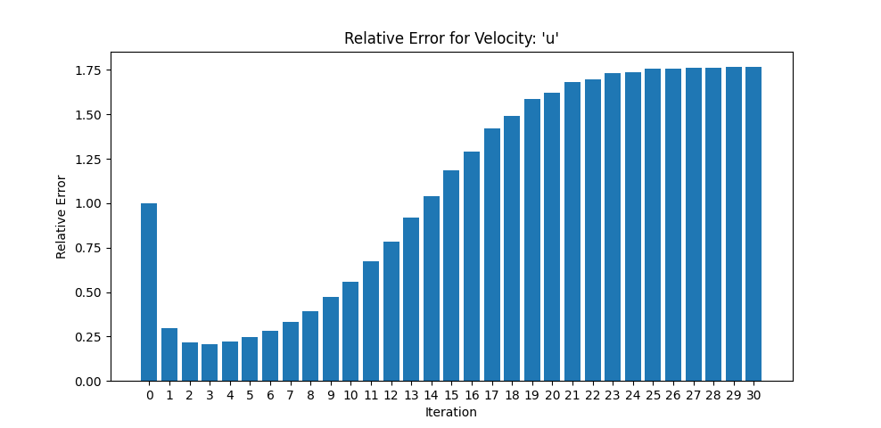
• After observations on the iteration limit, one more condition is added such that if relative error starts to grow breaks the loop. Max iteration size is no longer an important parameter thanks to this condition.

Reference Paper

[1] Horn and Schunck. (1981). Determining Optical Flow

Credits

Utilized from OpticalFlow_Visualization by Tom Runia (tomrunia@github) for optical flow field colorization.

Gauss Seidel Approach and Relative Error

In the reference paper, Gauss Seidel approach is proposed to solve the convex optimization problem. However, it is a bit tricky way here that next flow velocities are not directly depend on previous values, but its Laplacian.

This method can not allow us to calculate absolute error; therefore, relative error is used. For simplification, only flow matrix u is computed due to same characteristics with v matrix. Also, mean of the matrices are used to reach a scalar value. Below code sample shows how relative error is calculated in this project; where, u is the new calculated matrix and self.u previous.

 e = np.mean(np.absolute(u-self.u)) / np.mean(np.absolute(u)) 

Inference

It is clearly seen in above observation that there is a strong correlation between iteration number and flow field accuracy. The best optical flow vectors generated with 3 iterations which has the lowest relative error, in this example. Consequently, one more condition is added such that if relative error starts to grow breaks the Gauss Seidel loop, as an inference.

Horn and Schunck Smoothness Constraint

Smoothing parameter, alpha, is the regularization coefficient of the smoothness constraint in the Horn and Schunck optimization equation. Alpha is the measurement of the effect of smoothness constraint on the error term. This constraint forces flow velocities u and v to be less variable or more stable both in changing area and also time.

Effects on the Accuracy of the Flow Field and Prediction

Greater alpha resulted in the orientations of the flow velocities to be almost same in the close neighbor area. This can be observed as more intense colors on the flow field. To illustrate, train object appears in more stable red color and calendar purple over growing alpha value, see this section. Keep in mind that down oriented flow vectors shown in purple, up is yellow, right is green and left is red as color codes.

Additionally, more accurate flow field estimates lets the prediction also be more accurate. The predicted video can be considered as the twin of the ground truth for the alpha value equals to 100, see this section.